
Data & Vinyls — A discogs library exploration with R
As a vinyl lover and data addict, I had some fun making requests on the Discogs API with R, in order to know better what is inside my library.
Every vinyl lover knows about Discogs. But did you know you could easily access the API? Here are the lines of code I used to access my library.
Note : You can download the data used here in JSON, or directly in R :
collection_complete <- jsonlite::fromJSON(txt = "http://colinfay.me/data/collection_complete.json", simplifyDataFrame = TRUE)
Major Tom to Discogs API
Before starting, I’ll need these two functions: _
%>% and ` %||%`._
library(magrittr) #for %>%
`%||%` <- function(a,b) if(is.null(a)) b else a
Let’s first get my Discogs profile:
user <- "_colin"
content <- httr::GET(paste0("https://api.discogs.com/users/", user, "/collection/folders"))
content <- rjson::fromJSON(rawToChar(content$content))$folders
content
## [[1]]
## [[1]]$count
## [1] 308
##
## [[1]]$resource_url
## [1] "https://api.discogs.com/users/_colin/collection/folders/0"
##
## [[1]]$id
## [1] 0
##
## [[1]]$name
## [1] "All"
This first request brings in the environment all the information about a profil (here “_colin”, aka : me).
$count
``` tells us the number of entries in the library : 308. The ```r
$id
``` element is the number of “folders” created by the user – 0 corresponding to the whole collection, without any list specification.
### Create a dataframe with all the vinyls
The Discogs API sends back pages with 100 max results. Here, my collection has 308, so I'll use a ```r
repeat
``` loop to query all the data, and store them in a dataframe.
```r
collec_url <- httr::GET(paste0("https://api.discogs.com/users/", user, "/collection/folders/", content[[1]]$id, "/releases?page=1&per_page=100"))
if (collec_url$status_code == 200){
collec <- rjson::fromJSON(rawToChar(collec_url$content))
collecdata <- collec$releases
if(!is.null(collec$pagination$urls$`next`)){
repeat{
url <- httr::GET(collec$pagination$urls$`next`)
collec <- rjson::fromJSON(rawToChar(url$content))
collecdata <- c(collecdata, collec$releases)
if(is.null(collec$pagination$urls$`next`)){
break
}
}
}
}
collection <- lapply(collecdata, function(obj){
data.frame(release_id = obj$basic_information$id %||% NA,
label = obj$basic_information$labels[[1]]$name %||% NA,
year = obj$basic_information$year %||% NA,
title = obj$basic_information$title %||% NA,
artist_name = obj$basic_information$artists[[1]]$name %||% NA,
artist_id = obj$basic_information$artists[[1]]$id %||% NA,
artist_resource_url = obj$basic_information$artists[[1]]$resource_url %||% NA,
format = obj$basic_information$formats[[1]]$name %||% NA,
resource_url = obj$basic_information$resource_url %||% NA)
}) %>% do.call(rbind, .) %>%
unique()
Here is what the dataframe looks like:
library(pander)
pander(head(collection))
| release_id | label | year | title |
|---|---|---|---|
| 5181773 | A&M Records | 1982 | Night And Day |
| 3690646 | A&M Records (2) | 2012 | God Save The Queen |
| 944917 | Alexi Delano Limited | 2007 | The Acid Sessions Vol. 4 |
| 906983 | Alphabet City | 2007 | Urban Minds / Skattered |
| 8112758 | Amerilys | 1986 | Follement Vôtre |
| 5800664 | Anette Records | 2014 | And The Dead Shall Lie There |
| artist_name | artist_id | artist_resource_url | format |
|---|---|---|---|
| Joe Jackson | 75280 | https://api.discogs.com/artists/75280 | Vinyl |
| Sex Pistols | 31753 | https://api.discogs.com/artists/31753 | Vinyl |
| Alexi Delano | 26 | https://api.discogs.com/artists/26 | Vinyl |
| Pacjam | 488187 | https://api.discogs.com/artists/488187 | Vinyl |
| Diane Dufresne | 647100 | https://api.discogs.com/artists/647100 | Vinyl |
| Ancient Mith | 302464 | https://api.discogs.com/artists/302464 | Vinyl |
I can’t see, I can’t see I’m going blind
And now, let’s start visualising!
Most frequent labels
library(ggplot2)
ggplot(as.data.frame(head(sort(table(collection$label), decreasing = TRUE), 10)), aes(x = reorder(Var1, Freq), y = Freq)) +
  geom_bar(stat = "identity", fill = "#B79477") +
  coord_flip() +
  xlab("Label") +
  ylab("Fréquence") +
  ggtitle("Labels les plus fréquents")
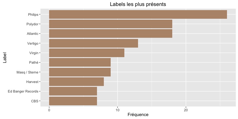
Philips and Polydor, what a surprise!
Most frequent artists
ggplot(as.data.frame(head(sort(table(collection$artist_name), decreasing = TRUE), 10)), aes(x = reorder(Var1, Freq), y = Freq)) +
  geom_bar(stat = "identity", fill = "#B79477") +
  coord_flip() +
  xlab("Artistes") +
  ylab("Fréquence") +
  ggtitle("Artistes les plus fréquents")
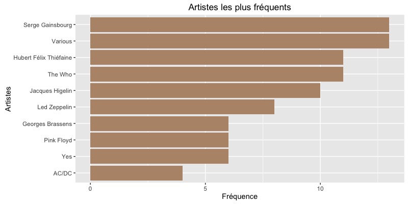
So… here’s the big revelation: I love Serge Gainsbourg and Geogres Brassens (guilty pleasure).
Release date
ggplot(dplyr::filter(collection, year != 0), aes(x = year)) +
  geom_bar(stat = "count", fill = "#B79477") +
  xlab("Année de sortie") +
  ylab("Fréquence") +
  ggtitle("Date de sorties des vinyles de la collection")
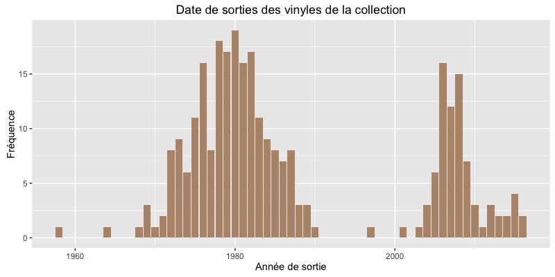
Looks like I’m not a big 90’s fan! My library show a bimodal distribution, with one mode around the 80’s, and one around 2005.
It’s time to go deeper
So, can we get more information about this library?
Hello, it’s me again
_Note: between the writing of this blogpost and now, Discogs seems to have put a rate limit on its API. For the creation of collection_2, you should consider using Sys.sleep(). More on that here.
collection_2 <- lapply(as.list(collection$release_id), function(obj){
  url <- httr::GET(paste0("https://api.discogs.com/releases/", obj))
  url <- rjson::fromJSON(rawToChar(url$content))
  data.frame(release_id = obj,
             label = url$label[[1]]$name %||% NA,
             year = url$year %||% NA,
             title = url$title %||% NA,
             artist_name = url$artist[[1]]$name %||% NA,
             styles = url$styles[[1]] %||% NA,
             genre = url$genre[[1]] %||% NA,
             average_note = url$community$rating$average %||% NA,
             votes = url$community$rating$count %||% NA,
             want = url$community$want %||% NA,
             have = url$community$have %||% NA,
             lowest_price = url$lowest_price %||% NA,
             country = url$country %||% NA)
}) %>% do.call(rbind, .) %>%
  unique()
Here, I have used the release_id element to make a request about each vinyl.
Most frequent genre
ggplot(as.data.frame(head(sort(table(collection_2$genre), decreasing = TRUE), 10)), aes(x = reorder(Var1, Freq), y = Freq)) +
  geom_bar(stat = "identity", fill = "#B79477") +
  coord_flip() +
  xlab("Genre") +
  ylab("Fréquence") +
  ggtitle("Genres les plus fréquents")
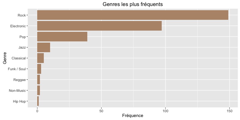 OH GOD, what a surprise! Almost half of my collection is made of rock albums (who could have guessed?).
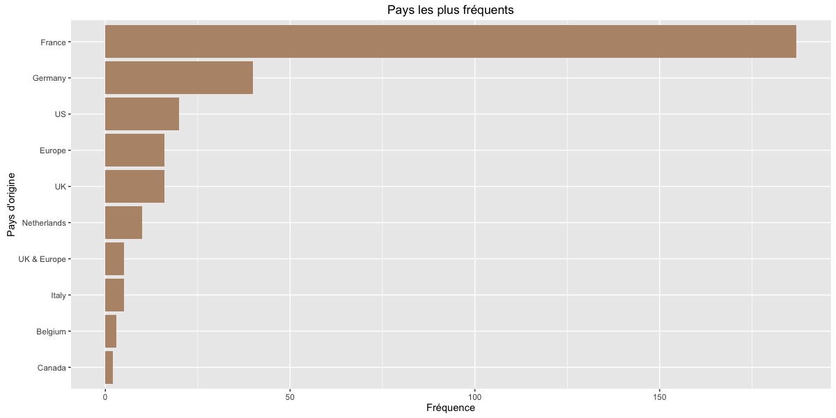
Countries
ggplot(as.data.frame(head(sort(table(collection_2$country), decreasing = TRUE), 10)), aes(x = reorder(Var1, Freq), y = Freq)) +
  geom_bar(stat = "identity", fill = "#B79477") +
  coord_flip() +
  xlab("Pays d'origine") +
  ylab("Fréquence") +
  ggtitle("Pays les plus fréquents")
Average note
ggplot(collection_2, aes(x = average_note)) +
  geom_histogram(fill = "#B79477") +
  xlab("Note moyenne") +
  ylab("Fréquence") +
  ggtitle("Notes moyennes des vinyles de la collection")

Thanks a lot Discogs! It looks like I’ve got quite good musical tastes (thanks for the ego boost :) !)
Prices of vinyls (low range)
ggplot(collection_2, aes(x = lowest_price)) +
  geom_histogram(fill = "#B79477") +
  xlab("Prix le plus bas") +
  ylab("Fréquence") +
  ggtitle("Prix le plus bas des vinyles de la collection")
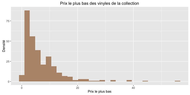
Ok, I’m not gonna be rich selling my vinyl collection…
Let’s finish!
collection_complete <- merge(collection, collection_2, by = c("release_id","label", "year", "title", "artist_name"))
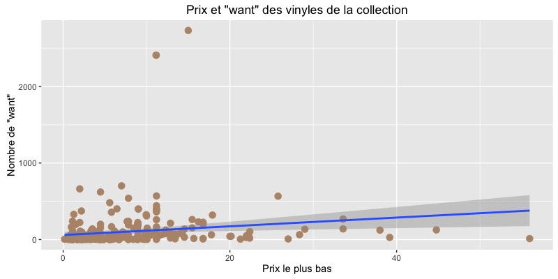
Relationship between price and “want”
lm_want <- lm(formula = lowest_price ~ want, data = collection_complete)
summary(lm_want)
##Residuals:
##   Min     1Q Median     3Q    Max
##-8.043 -4.628 -2.224  2.179 49.608

##Coefficients:
##            Estimate Std. Error t value Pr(>|t|)
##(Intercept) 6.715418   0.450582  14.904  < 2e-16 ***
##want        0.005004   0.001788   2.799  0.00546 **
##---
##Signif. codes:  0 ‘***’ 0.001 ‘**’ 0.01 ‘*’ 0.05 ‘.’ 0.1 ‘ ’ 1

##Residual standard error: 7.306 on 301 degrees of freedom
##  (5 observations deleted due to missingness)
##Multiple R-squared:  0.02536,    Adjusted R-squared:  0.02213
##F-statistic: 7.833 on 1 and 301 DF,  p-value: 0.005461
Here, we can see a correlation between the price and the number of users that put a “want” on a particular vinyl.
ggplot(collection_complete, aes(x = lowest_price, y = want)) + geom_point(size = 3, color = "#B79477") + geom_smooth(method = "lm") + xlab("Prix le plus bas") + ylab("Nombre de \"want\"") + ggtitle("Prix et \"want\" des vinyles de la collection")
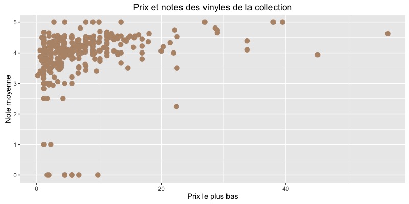
Price and average note
lm_note <- lm(formula = lowest_price ~ average_note, data = collection_complete)
lm_note$coefficients
##  (Intercept) average_note
##    -1.504767     2.207834
Here, no significative correlation.
ggplot(collection_complete, aes(x = lowest_price, y = average_note)) +
  geom_point(size = 3, color = "#B79477") +
  xlab("Prix le plus bas") +
  ylab("Note moyenne") +
  ylim(c(0,5)) +
  ggtitle("Prix et notes des vinyles de la collection")
And to conclude…
Next step… create a package to access the Discogs API? Why not! Let’s put this on my to-do…
What do you think?