2018 through {cranlogs}

2018 at glance with {cranlogs}.

Let’s load the necessary packages.

library(cranlogs)
library(data.table)
library(lubridate)

## 
## Attaching package: 'lubridate'

## The following objects are masked from 'package:data.table':
## 
##     hour, isoweek, mday, minute, month, quarter, second, wday,
##     week, yday, year

## The following object is masked from 'package:base':
## 
##     date

library(ggplot2)
library(magrittr)

All downloads

We’ll use {cranlogs} to retrieve the data from the RStudio CRAN mirror.

First, the number of package downloads by day in 2018.

total_dl <- cran_downloads(from = "2018-01-01", to = "2018-12-31")

# Turn to a data.table
setDT(total_dl)

# Round the date to month and week
total_dl[, `:=`(
  round_week = floor_date(date, "week" ),
  round_month = floor_date(date, "month" )
  ) ]

How many download in total?

total_dl[, .(total = sum(count))]

##        total
## 1: 614548197

Let’s plot this:

random_viridis <- function(n){
  sample(viridis::viridis(100), n)
}
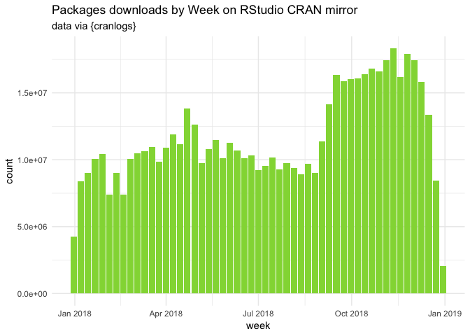
total_dl[, .(count = sum(count)), round_week] %>%
  ggplot(aes(round_week, count)) + 
  geom_col(fill = random_viridis(1)) + 
  labs(
    title = "Packages downloads by Week on RStudio CRAN mirror", 
    subtitle = "data via {cranlogs}", 
    x = "week"
  ) + 
  theme_minimal()

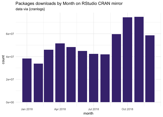
total_dl[, .(count = sum(count)), round_month] %>%
  ggplot(aes(round_month, count)) + 
  geom_col(fill = random_viridis(1)) + 
  labs(
    title = "Packages downloads by Month on RStudio CRAN mirror", 
    subtitle = "data via {cranlogs}", 
    x = "month"
  ) + 
  theme_minimal()

R download

Let’s now have a look at the number of downloads for R itself:

total_r <- cran_downloads("R", from = "2018-01-01", to = "2018-12-31")

setDT(total_r)

total_r[, `:=`(
  round_week = floor_date(date, "week" ),
  round_month = floor_date(date, "month" )
) ]

How many download in total?

total_r[, .(total = sum(count))]

##      total
## 1: 1041727

Plotting this:

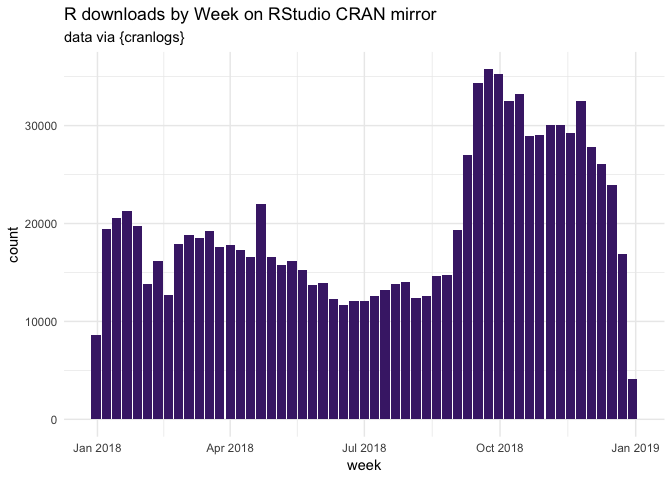
total_r[, .(count = sum(count)), round_week] %>%
  ggplot(aes(round_week, count)) + 
  geom_col(fill = random_viridis(1)) + 
  labs(
    title = "R downloads by Week on RStudio CRAN mirror", 
    subtitle = "data via {cranlogs}", 
    x = "week"
  ) + 
  theme_minimal()

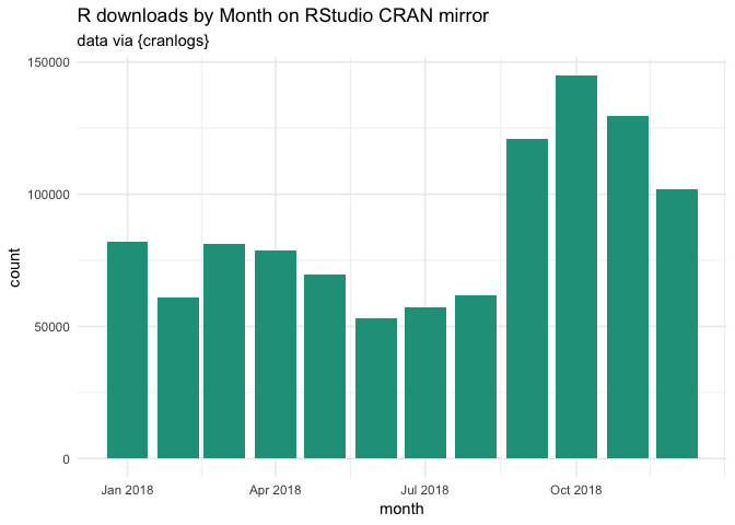
total_r[, .(count = sum(count)), round_month] %>%
  ggplot(aes(round_month, count)) + 
  geom_col(fill = random_viridis(1)) + 
  labs(
    title = "R downloads by Month on RStudio CRAN mirror", 
    subtitle = "data via {cranlogs}", 
    x = "month"
  ) + 
  theme_minimal()

Let’s have a look to the number of download by R version:

total_r[, .(count = sum(count)), version][order(count, decreasing = TRUE)] %>%
  head(10)

##          version  count
##  1:        3.5.1 464837
##  2:        3.4.3 174665
##  3:        3.5.0 137886
##  4:        3.4.4 107124
##  5:       latest  32642
##  6: 3.5.1patched  32119
##  7:        3.3.3  27992
##  8:        3.5.2  21645
##  9:        devel   8543
## 10:        3.2.4   4814

total_r[, .(count = sum(count)), version][order(count)] %>%
  head(10)

##        version count
##  1:    3.5.1rc     2
##  2:  3.5.2beta     2
##  3:    3.5.2rc     6
##  4:  3.5.0beta     8
##  5:    3.4.4rc    11
##  6: 3.5.0alpha    11
##  7:    3.5.0rc    12
##  8:      2.6.1    13
##  9:      2.8.0    16
## 10:      2.2.1    17

total_r[, .(count = sum(count)), version][order(count, decreasing = TRUE)] %>%
  head(10) %>% 
  ggplot(aes(reorder(version, count), count)) +
  coord_flip() +
  geom_col(fill = random_viridis(1)) + 
  labs(
    title = "10 most downloaded R versions in 2018 on RStudio CRAN mirror", 
    subtitle = "data via {cranlogs}", 
    x = "version"
  ) + 
  theme_minimal()

And by os:

total_r[, .(total = sum(count)), os]

##     os  total
## 1: osx 228573
## 2: win 767319
## 3: src  42725
## 4:  NA   3110

And a happy new year 🎉🎉